
Chapter 3: Location, Location, Location
Adapted from Fang
Location-based analyses distinguished geography from other fields. Location is the key to accessing geospatial research. There are many ways to describe location.
Shape of the Earth
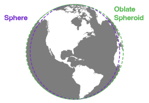
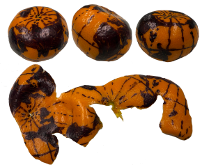
The Earth’s constant spinning causes it to bulge slightly along the equator, ruining its perfect spherical shape; it’s a geoid with a slight pear shape; it is a little larger in the southern hemisphere and includes other bulges. The slightly oval nature of the Earth’s geometric surface makes the terms ellipsoid and oblate spheroid more accurate in describing its shape, but they are not perfect terms either due to differences in material weights (for instance iron is denser than sedimentary deposits), and the movement of tectonic plates makes the Earth dynamic and constantly changing.
Absolute Location
This is precise position on the surface of the Earth, most often expressed as coordinate pairs (Latitude and Longitude). Global positioning systems (GPS) can determine absolute coordinates on Earth. GPS technology consists of a constellation of satellites that are orbiting the earth and constantly transmitting time signals. To determine a position, earth-based GPS units (e.g., handheld devices, car navigation systems, mobile phones) receive the signals from at least three of these satellites and use this information to triangulate a location. All GPS units use the geographic coordinate system (GCS) to report location. Location can also be expressed as an address. Addresses can be brought into a GIS through a process called geocoding, which uses an existing reference dataset, or a locator, to match an address to a location.
Nominal Location
Nominal location refers to named geographic features or place names; these locations can be cities, countries, administrative names (e.g., Siberia), or natural features (e.g., Rocky Mountains). Place names are organized in gazetteers, the most standardly used gazetteer is Geonames. Gazetteers can also be used as a locator to bring place names into a GIS.
Relative Location
Location can also be defined in relative terms. Relative location refers to defining and describing places in relation to other known locations. For instance, Cairo, Egypt, is north of Johannesburg, South Africa; New Zealand is southeast of Australia; and Kabul, Afghanistan, is northwest of Lahore, Pakistan. Unlike nominal or absolute locations that define single points, relative locations provide a bit more information and situate one place in relation to another.
Direction
Direction can be used a benchmark to establish relative location. South Poles serve as the geographic benchmarks for determining direction. Magnetic north (and south) refers to the point on the surface of the earth where the earth’s magnetic fields converge. This is also the point to which magnetic compasses point. Note that magnetic north falls somewhere in northern Canada and is not geographically coincident with true north or the North Pole. Grid north simply refers to the northward direction that the grid lines of latitude and longitude on a map, called a graticule.
Geographic Coordinate System (Latitude, Longitude)
A geographic coordinate systems measure the spherical Earth based on a common datum. This measurement is expressed in coordinate pairs, latitude and longitude. Earth’s center to a point on the Earth’s surface.
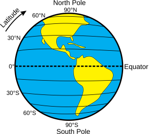
Latitude
Across the spherical Earth, latitude lines (parallels) stretch horizontally from east to west, and they are parallel to each other, hence their alternative name, parallels. Latitude can be thought of as the lines that intersect the y-axis, and longitude as lines that intersect the x-axis.
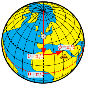
Longitude

Longitude lines (meridians) stand vertically and stretch from the North Pole to the South Pole. The y axis is the prime meridian, which is a line running from pole to pole through Greenwich, England.
Together these “north to south” and “east to west” lines meet at perpendicular angles to form a graticule, a grid that encompasses the Earth. Just as the upper right quarter in the Cartesian coordinate system is positive for both x and y, latitude and longitude east of the prime meridian and north of the equator are both positive.
+/-
Europe, Asia, and part of Africa – which have positive latitudes and longitudes – correspond to the upper right quarter of the Cartesian coordinate system. With the exception of some U.S. territories in the Pacific and the westernmost Aleutian Islands, all of the United States is north of the equator and west of the prime meridian, so all latitudes in the U.S are positive (or north) while almost all longitudes are negative (or west).
Midway between the poles, the equator stretches around the Earth, and it defines the line of zero degrees latitude. Relative to the equator, latitude is measured from 90 degrees at the North Pole to –90 degrees at the South Pole. Prime Meridian is the line of zero degrees longitude, and in most coordinate systems, it passes through Greenwich, England. Longitude runs from -180 degrees west of the Prime Meridian to 180 degrees east of the same meridian. Because the globe is 360 degrees in circumference, -180 and 180 degrees is the same location.
Datum
All coordinate systems are measured relative to a datum. A datum defines the starting point from which coordinates are measured. Latitude and longitude coordinates, for example, are determined by their distance from the equator and the prime meridian that runs through Greenwich, England. But where exactly is the equator? And where exactly is the Prime Meridian? And how does the irregular shape of the Earth figure into our measurements? All of these issues are defined by the datum. Many different datums exist, but in the United States only three datums are commonly used.
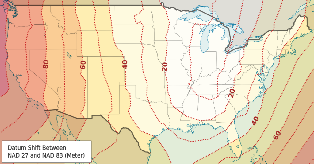
- NAD 27: The North American Datum of 1927 (NAD27) uses a starting point at a base station in Meades Ranch, Kansas and the Clarke Ellipsoid to calculate the shape of the Earth.
- NAD 83: Thanks to the advent of satellites, a better model later became available and resulted in the development of the North American Datum of 1983 (NAD83). Depending on one’s location, coordinates obtained using NAD83 could be hundreds of meters away from coordinates obtained using NAD27.
- WGS 84: A third datum with a starting point in Greenwich, England, the World Geodetic System of 1984 (WGS84) is identical to NAD83 for most practical purposes within the United States. The differences are only important when an extremely high degree of precision is needed. WGS84 is the default datum setting for almost all GPS devices and web maps. But most USGS topographic maps published up to 2009 use NAD27.
Projection (Transformation of Geographical Coordinates to Cartesian Coordinate Systems)
While the system of latitude and longitude provides a consistent referencing system for anywhere on the earth, to portray our information on maps or for making calculations, we need to transform these angular measures to Cartesian coordinates. These transformations amount to a mapping of geometric relationships expressed on the shell of a globe to an attenable surface — a mathematical problem.
Why project
Globes do not need projections, and even though they are the best way to depict the Earth’s shape and to understand latitude and longitude, they are not practical for most applications that require maps. We most often experience 2D maps, whether physical or digital; reshaping a globe requires a mathematical reshaping of the Earth’s 3-dimensions into a 2-dimensional surface.
To illustrate the concept of a map projection, imagine that we place a light bulb in the center of a translucent globe.
On the globe are outlines of the continents and the lines of longitude and latitude called the graticule. When we turn the light bulb on, the outline of the continents and the graticule will be “projected” as shadows on
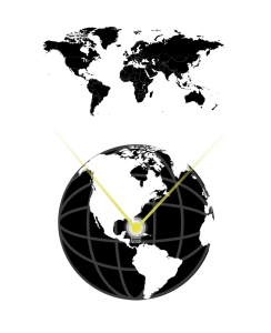
the wall, ceiling, or any other nearby surface. This is what is meant by map “projection.” The term projection implies that the ball-shaped net of parallels and meridians is transformed by casting its shadow upon some ‘at, or ‘attenable, surface. In fact, almost all map projection methods are mathematical equations. The projected graticule produced by projection equations in each category. Referring again to the previous example of a light bulb in the center of a globe, note that during the projection process, we can situate each surface in any number of ways. For example, surfaces can be tangential to the globe along the equator or poles, they can pass through or intersect the surface, and they can be oriented at any number of angles. As you might imagine, the appearance of the projected grid will change quite a lot depending on the type of surface it is projected onto, and how that surface is aligned with the globe. The following figures shows how these projections can vary.
Why Not to Project: Small Study Area
If the geographic extent of your project area was small, like a neighborhood or a portion of a city, you could assume that the Earth is that and use no projection. This is referred to as a planar surface or even a planar “projection,” but with the understanding that it does not use a projection. Planar representation does not significantly affect a map’s accuracy when scales are larger than 1:10,000. In other words, small areas do not need a projection because the statistical differences between locations on a flat plane and a 3-dimensional surface are not significant. For small-scale maps one must consider the Earth’s shape. Our assumption that the Earth is round or spherical does not accurately represent it.
Projection Categories:
Within the realm of maps and mapping, there are three surfaces used for map projections (i.e., surfaces on which we project the shadows of the graticule). These surfaces categories are:
Cylindrical

- straight coordinate lines
- horizontal parallels crossing meridians at right angles
- all meridians are equally spaced
- the scale is consistent along each parallel
Conic
The cone is typically aligned with the globe such that its line of contact (tangency) coincides with a parallel in the mid-latitudes:
- meridians are equidistant & straight lines
- converge in locations regardless of presence of a pole
- parallels cross the meridians at right angles
- constant measure of distortion throughout
Planar (Azimuthal)
The planar is centered upon a specific point and perspective and is frequently positioned tangent to the equator:
- the point can be based on the poles (stereographic), the equator (gnomic) or from a defined oblique point (orthographic).
- a point specifies the focused of projection identified by a central coordinate
- polar projections are most straightforward, and often cited
- meridian and parallels intersect at their true position
- most accurate at the focal point, patterns of distortion move out from it in straight line measurement creation “great circles”.
Projection and Distortion
Flattening the globe cannot be done without introducing some error, and some distortion is unavoidable. Any projection has its area of least distortion. Projections can be shifted around to put this area of least distortion over the topographer’s area of interest. Thus, any projection can have an unlimited number of variations or cases that determined by standard parallels or meridians that adjust the location of the high-accuracy part of the projection.
Projections are abstractions, and they introduce distortions to either the Earth’s shape, area, distance, or direction (and sometimes to all of these properties).
Within each projection family there are many different projections to choose from. All of them create distortion in one manner or another. Determining what needs to be preserved about your study area is the first step. Map projections are often classified by the characteristic they do not distort. Usually only one property is preserved in a projection.
Classifications
- Conformal – preserves shape, and distorts area
- Equal Area – preserves: area, distorts shape, scale, or angle (bearing)
- Equidistant – preserves distances between certain points (but not all points) and distorts other distances
Conformal
Conformal map projections are used for navigational purposes due to the importance of maintaining a bearing or heading when traveling great distances. The cost of preserving bearings is that areas tend to be quite distorted in conformal map projections. Although shapes are more or less preserved over small areas, at small scales areas become wildly distorted.
The Mercator projection is an example of a conformal projection and is famous for distorting Greenland. As the name indicates, equal area or equivalent projections preserve the quality of area. Such projections are of particular use when accurate measures or comparisons of geographical distributions are necessary (e.g., deforestation, wetlands). To maintain true proportions in the surface of the earth, features sometimes become compressed or stretched depending on the orientation of the projection. Moreover, such projections distort distances as well as angular relationships.
Equal Area
This projection type is focused on preserving area at the cost of everything else. This means shape can often be distorted. Equal area is commonly used for thematic mapping. Their advantage is in most accurately representing distributions.
Azimuthal Equidistant projection (planar, orthographic). The focal point is Taipei in Taiwan. Projection is most accurate near to the focal point but becomes distorted as it circles out to the greater world.
-
- Great Circles:
- Red circle: 10,000 km distance
- Purple circle: 15,000 km distance
- Distorted Countries:
- Yellow – Brazil
- Pink – Argentina
- Gray – Uruguay
- Orange – Paraguay
- Green – Chile
- Violet – Bolivia
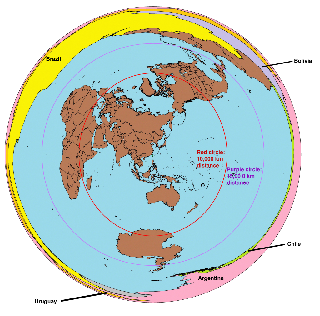
Illustration of Azimuthal Equidistant projection
- Great Circles:
The Albers (conic) projection is a common equal area projection using two standard parallels which ensures area is preserved between them. This projection is common in environmental and governmental maps.
Equidistant
Map projections that accurately represent distances are referred to as equidistant projections. Note that distances are only correct in one direction, usually running north–south, and are not correct everywhere across the map. Equidistant maps are frequently used for small-scale maps that cover large areas because they do a good job of preserving the shape of geographic features such as continent.
- Azimuthal Equidistant is a common projection for mapping small areas.
Choosing the right projection
As noted earlier, there are theoretically an infinite number of map projections to choose from. One of the key considerations behind the choice of map projection are to reduce the amount of distortion. The geographical object being mapped and the respective scale at which the map will be constructed are also important factors to think about. For instance:
- Maps of the North and South Poles usually use planar or azimuthal projections, and conical projections are best suited for the middle latitude areas of the earth.
- Features that stretch east–west, such as the country of Russia, are represented well with the standard cylindrical projection
- Countries which are oriented north–south (e.g., Chile, Norway) are better represented using a transverse projection.
If a map projection is unknown, sometimes it can be identified by working backward and examining closely the nature and orientation of the graticule (i.e., grid of latitude and longitude), as well as the varying degrees of distortion. Clearly, there are trade-offs made regarding distortion on every map.
- There are no hard-and-fast rules as to which distortions are more preferred over others.
- The selection of map projection largely depends on the purpose of the map.
Within the scope of GISs, knowing and understanding map projections is critical. For instance, to perform an overlay analysis, all map layers need to be in the same projection. If they are not, geographical features will not be aligned properly, and any analyses performed will be inaccurate and incorrect. If you want to conduct a measurement of land parcel size, you need to use a projection that does not distort area space. Most GISs include functions to assist in the identification of map projections, as well as to transform between projections to synchronize geospatial data. Despite the capabilities of technology, an awareness of the potential and pitfalls that surround map projections is essential.
On the Fly Projection
In a GIS the first dataset added to a project sets the coordinate system; subsequent layers are transformed to display in the projection of the first dataset. It should be noted that this is not a true reprojection, and any changes made to the dataset, or any comparisons made to other layers when it’s displayed in an on-the-fly projection are likely to create errors. It’s recommended that data be projected properly before editing or analyzing.
Although projecting a dataset was once incredibly difficult, today, we can project and reproject massive quantities of coordinates, transforming them backward and forward from Latitude and Longitude to overlay precisely with data that are stored in some other coordinate space. Automatic transformation of coordinate systems requires that datasets include machine-readable metadata. In about 2002, the makers of ArcMap made projection on the fly possible when it added one a new file to the schema of a shapefile; the .prj file, which contains the description of the projection of a shapefile, and if it exists, it is always copied with the shape file or elements that are exported from it. This is the machine-readable metadata that allowed ArcMap to know how to handle the dataset if any transformation (reprojection) is required; including projection metadata is now standardly stored in the data. There are plenty of datasets that do not include such machine-readable metadata so it’s important to know how to identify it when needed. Most GIS have the ability to project on-the-fly today.
Commonly used Projections
The Universal Transverse Mercator grid is commonly referred to as UTM and is based on the Transverse Mercator projection. Universal Transverse Mercator (UTM) is a coordinate system that largely covers the globe. The system reaches from 84 degrees north to 84 degrees south latitude, and it divides the Earth into 60 north-south oriented zones that are 6 degrees of longitude wide. The UTM system is not a single map projection.

- Transformation: The system instead 60 projections, and each uses a secant (a trigonometric function that for an acute angle is the ratio of the hypotenuse of a right triangle of which the angle is considered part and the leg adjacent to the angle) transverse Mercator projection in each zone.
- Zones: The contiguous U.S. consists of 10 zones: UTM zones are numbered consecutively beginning with Zone 1. Zone 1 covers 180 degrees west longitude to 174 degrees west longitude (6 degrees of longitude) and includes the westernmost point of Alaska. Maine falls within Zone 16 because it lies between 84 degrees west and 90 degrees west. In each zone, coordinates are measured as northings and eastings in meters.
- Central Meridian: The central meridian in each zone is assigned an easting value of 500,000 meters. In Zone 16, the central meridian is 87 degrees west. One meter east of that central meridian is 500,001 meters easting.
- Northing/False Northing: In the Northern hemisphere, the equator is the zero baseline for Northings (Southern hemisphere uses a 10,000 km false Northing).
- Easting/False Easting: Each zone has an arbitrary central meridian of 500 km west of each zone’s central meridian (called a false Easting) to insure positive Easting values and a central bisecting meridian.
State Plane Coordinate System
The State Plane Coordinate System is a series of separate systems, each covering a state, or a part of a state, and is only used in the United States. It is popular with some state and local governments due to its high accuracy, achieved using relatively small zones. State Plane began in 1933 with the North Carolina Coordinate System and in less than a year it had been copied in all the other states.
Accuracy: The system is designed to have a maximum linear error of 1 in 10,000 and is four times as accurate as the UTM system.
Zones: Like the UTM system, the State Plane system is based on zones. However, the 120 State Plane zones generally follow county boundaries (except in Alaska).
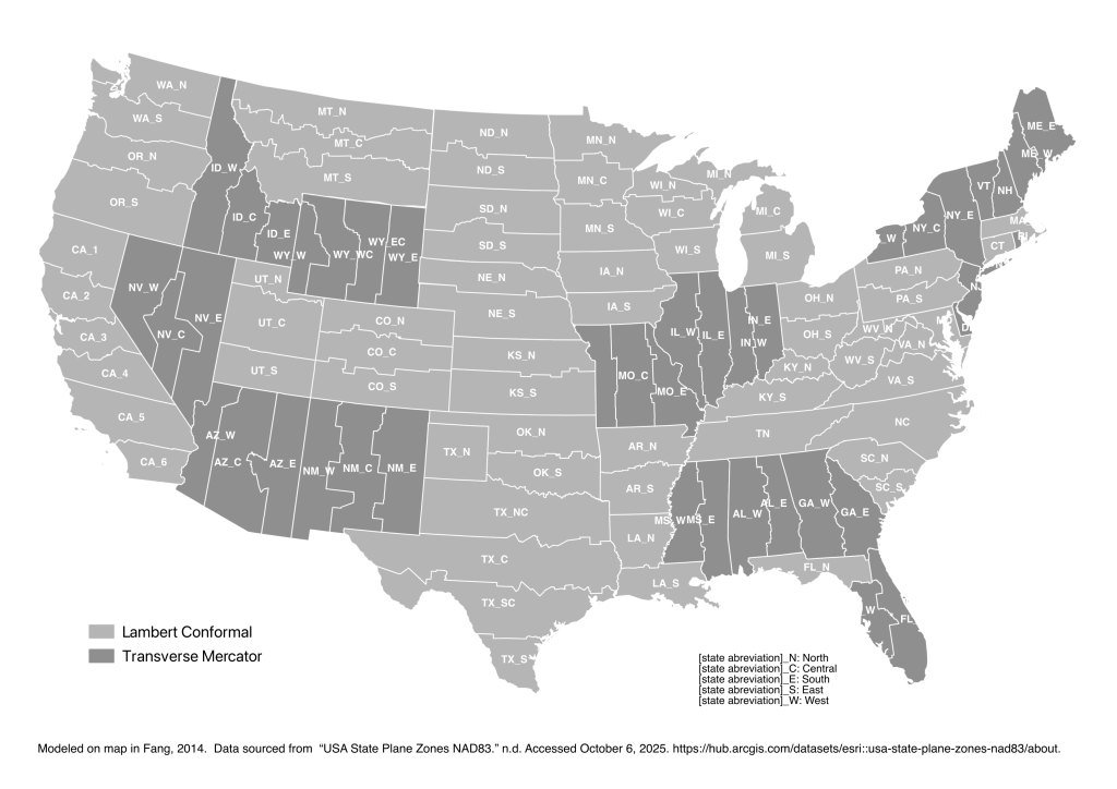
State Divisions: Given the State Plane system’s desired level of accuracy, larger states are divided into multiple zones, such as the “Colorado North Zone.”Transverse Mercator: States with a long north-south axis (such as Idaho and Illinois) are mapped using a Transverse Mercator projection,
Lambert Conformal: States with a long east-west axis (such as Washington and Pennsylvania) are mapped using a Lambert Conformal projection.[2]
Central meridian: In either case, the projection’s central meridian is generally run down the approximate center of the zone.
Positive Coordinates: A Cartesian coordinate system is created for each zone by establishing an origin at some distance (usually 2,000,000 feet) to the west of the zone’s central meridian and some distance to the south of the zone’s southernmost point. This ensures that all coordinates within the zone will be positive. The X-axis running through this origin runs east-west, and the Y-axis runs north-south.
Measurement: Distances from the origin are generally measured in feet but sometimes are in meters.
Eastings/Northings: X distances are typically called eastings (because they measure distances east of the origin) and Y distances are typically called northings (because they measure distances north of the origin).
Exercises
Exercise 3a. Convert DMS to DD
At times we come upon datasets in which the latitude and longitude are recorded in degrees, minutes, seconds (DMS), but for GIS having coordinates in decimal degrees is preferred. Data this dataset and convert the DMS coordinates to DD.
Formula: Decimal degrees = Degrees + (Minutes/60) + (Seconds/3600)
Dataset: download geothink_sdms.csv
Exercises
Exercise 3b. Find Your Local Projected Coordinate System
Find the projected coordinate system most appropriate for your local area.
