Chapter 12. Basic Data Management in QGIS
Data Management Tools
In this chapter, we’re going to learn some basic tools to get our data in shape for analysis. We prepared our tabular Census data in OpenRefine so that we’ll be able to take these steps in QGIS. Our first step is to join the prepared Census table to our tract data using a tabular join. By doing that we represent Census values quantitatively by location. Next we will create a spatial join to give our coffee, juice, bakery, ice cream location attributes from our municipal boundaries layer. We are doing this so the location is tied to its municipality. The locations came in as separate layers, but it might be easier to work with them as one layer so we will merge those datasets. To make it easier to categorize the locations, we’ll give them a new field were we can record their focus.
Step 1: Tabular Join
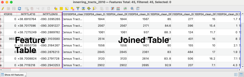
Once we have added our Census Tracts, we can join demographic data tables from the Census and visualize the values on the map.
Review of Requirements for a successful join
- Join fields must contain matching values (a unique identifier is an ideal value for joining)
- Join fields must be the same data format (e.g., string, integer, etc.)
- Field headers must not contain spaces or special characters
- Field values are clean and standardized
- Field headers should not use reserved words (e.g., date,” “day,” “month,” “table,” “text,” “user,” “when,” “where,” “year,” or “zone”)
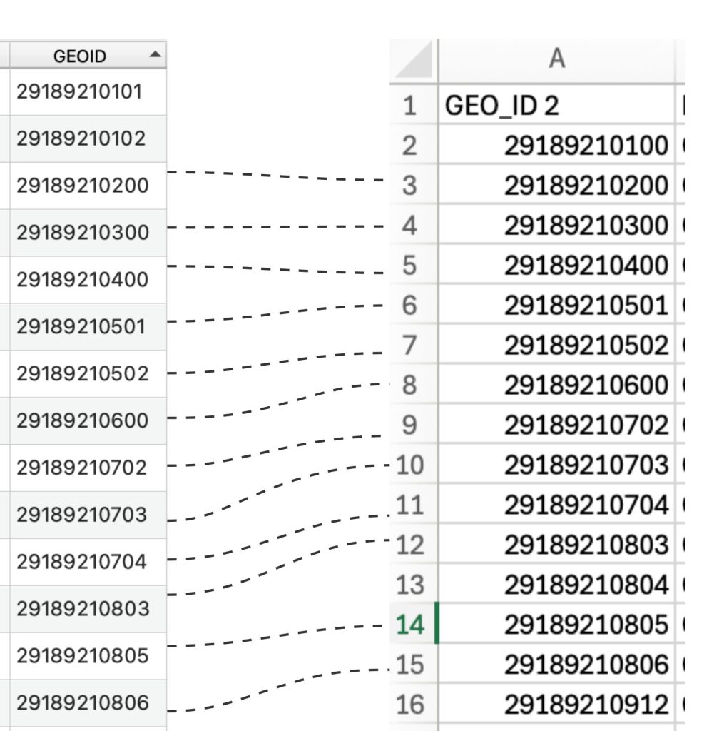
Join fields are often key fields in a table because they contain unique identifiers for each feature in the dataset. If our table has a field containing the unique identifiers that match the unique identifiers in the feature class, we can connect them.
1a. Add the census tables.
- Go to the data manager
- Add Delimited text
- Navigate DP04.csv
- Add to the project
- Repeat for:
- B02001.csv
- S1901.csv
1b. Join Income

- Right click on one of the innering_tracts layers
- Select properties
- Select Joins
- Click the plus sign and the join dialog appears
- Join layer: S1901.csv
- Join field: GEO_ID_2
- Target field: GEOID10
If the join failed, go back through the requirements and make sure your data meets them.
If the join succeeded but the values are null, go and check the requirements
Quickly symbolizing by graduated color can help you confirm the success of your join.
If you try to symbolize by graduated colors but don’t see your fields, it’s likely the software does not recognize your numbers as numeric, rather as numbers stored as text.
This often happens if row 2 has text in it. An easy solution is to add a dummy row two with a number in it.
This is necessary because we need our unique id column to read as numbers stored as text, but our value field to read as numbers stored as numbers. This dummy row will not affect the data because that field will not have a unique identifier and therefore will not join to the geospatial data. However, it is a good idea to note your dummy row in your documentation.
1c. Export layer as innerring_tract_income
1d. Remove join
- Right click on innerring_tracts
- Go to properties
- Joins
- Click the minus icon
- The join will be removed.
1d. One by one, join the other layers, and export them to their own layer.
Step 2: Spatial Join
- In QGIS, a spatial join appends attributes of one feature to another feature. We are going to append the inner ring municipalities to include which school district is serves that area. To do this, we must go to the vector menu in the top tool bar.
- Select Data Management
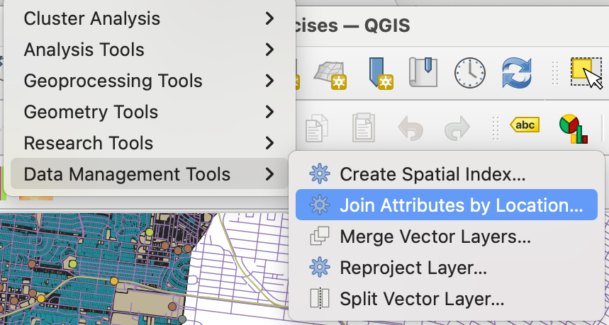
Screenshot of join by location in QGIS - Join Attributes by Location
- Join to Features in: innerring_muni
- Features they (geometric predicate): intersect
- By comparing to: innering_pubschools
- Fields to add: CityDist
- Joined layer: create temporary layer
- Run
- A temporary layer will be created
- Open the temporary layer, there should be a new column added to it called CityDist
- Some of the values will be null because they may not have a school district
- Check to make sure not all values are null
- Export layer, name it innerring_muni_sd
- Destination CRS: ESRI 102696 –NAD_StatePlane_Missouri_East_FIPS_2401_Feet
Step 3: Merge datasets
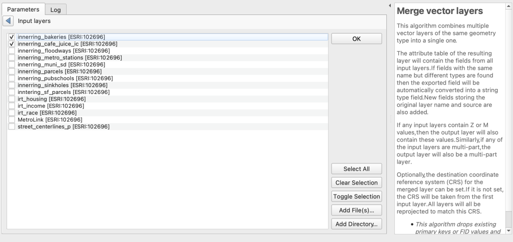
I would like the business locations to be in the same layer. To achieve this, we can use the merge vector layers tool
- Go to the Vector menu at the top
- Select Data management
- Select Merge Vector Layers
- Input layers: innerring_cafe_juice_ic; innerring_bakeries
- Destination CRS: ESRI 102696 – NAD_StatePlane_Missouri_East_FIPS_2401_Feet
- Merged: create temporary layer
- Run
- Open the attribute table, there should be 153 features in the new table (63 innerring_cafe_juice_ic plus 90 innerring_bakeries)
- Export merged layer:
- Save features as
- Navigate to your directory structure
- File name: innering_business
- CRS: ESRI 102696 – NAD_StatePlane_Missouri_East_FIPS_2401_Feet
- OK
Step 4: Add a new field
We might like to categorize the businesses by their specialty. Café, Bakery, Juice Bar, Ice Cream Shop. We can accomplish this by adding and populating a field.
Before adding the new field, I’m going to toggle off some the less helpful fields to ensure the table is easier to work with.
- Open the innerring_business layer’s attribute table
- Click the organize columns tool
- We will uncheck all the columns that are not serving our purpose; we can always toggle them on again if needed.
- Uncheck all fields except:
- Company
- City
- Layer
So we can easily distinguish between what the specialty of each location is, we will add field to categorize; this will allow us to parse the data by that category.
- Turn on (toggle) editing mode
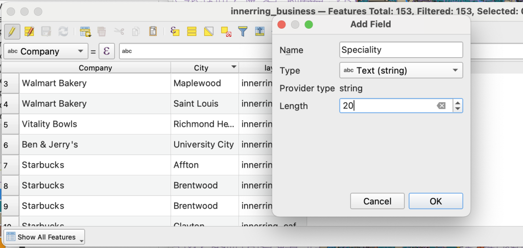
- Use the add field tool
- Name: Specialty
- Type: Text (string)
- Length: 20
- OK
- Be sure to save the edits in the table
Step 5: Create Value Mapping
Now we need to create standard values to keep the dataset tidy, also known as data validation.
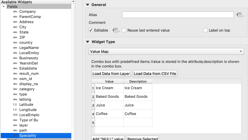
- Go to the layer properties
- Select Specialty from
- Choose the attribute form
- In the widget type box, change it to value map
- Add the values and descriptions. In our case, they are the same:
| Value | Description |
|---|---|
| Ice Cream | Ice Cream |
| Baked Goods | Baked Goods |
| Juice | Juice |
| Coffee | Coffee |
Now we can populate the table with standard values using a dropdown menu. We can use the layer type column to help us with Baked Goods, but otherwise we’ll need to look at the business name, in some cases we may need to google the name to be sure.

Step 6. Remove rows that don’t fit into a specialty that fits into our four groups.
- Example: Sugarfire specializes in barbecue
- Select the row in the table by clicking the box all the way to the left of each row
- Use delete tool in the table to remove the row/feature
- Save the edits in the table
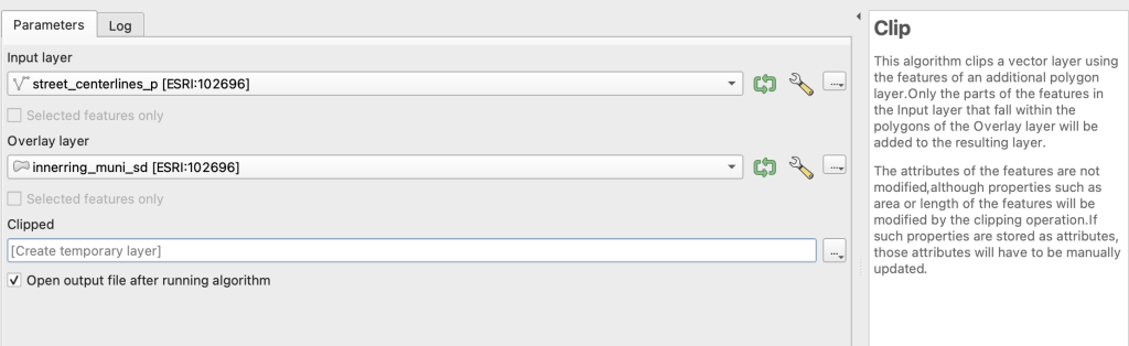
Step 7: Clip Street Centerlines
Now we will us a tool to clip out the St. Louis County parcels that are within the inner-ring municipalities.
- Turn of all the layers except the street_centerlines_p
- From the vector menu, select geoprocessing tools
- Choose the clip tool
- Input layer: parcels_2010
- Overlay layer: innerring_muni
- Clipped: Navigate to your folder, save as innerring_streets
- Check: open output file after running
- Run
Step 8: Edit Metrolink
Right click and open the attribute table on the Metrolink. Notice there’s not field distinguishing the Red Line (North West) and the (South West) Blue Line.
- Click the edit button
- Click the add field button
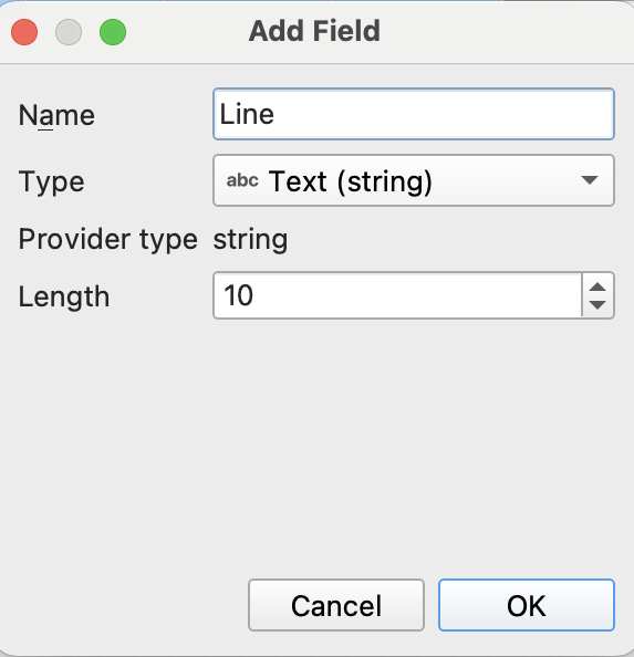
Screenshot of the add field dialog in QGIS - Name: Line
- Type: text
- Length: 10
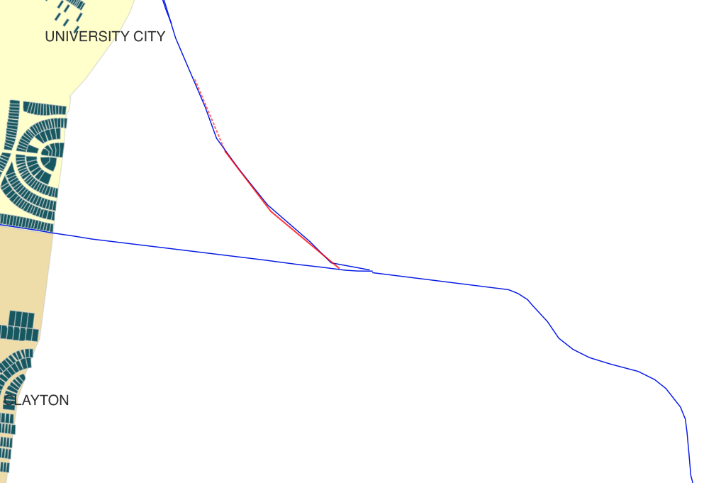
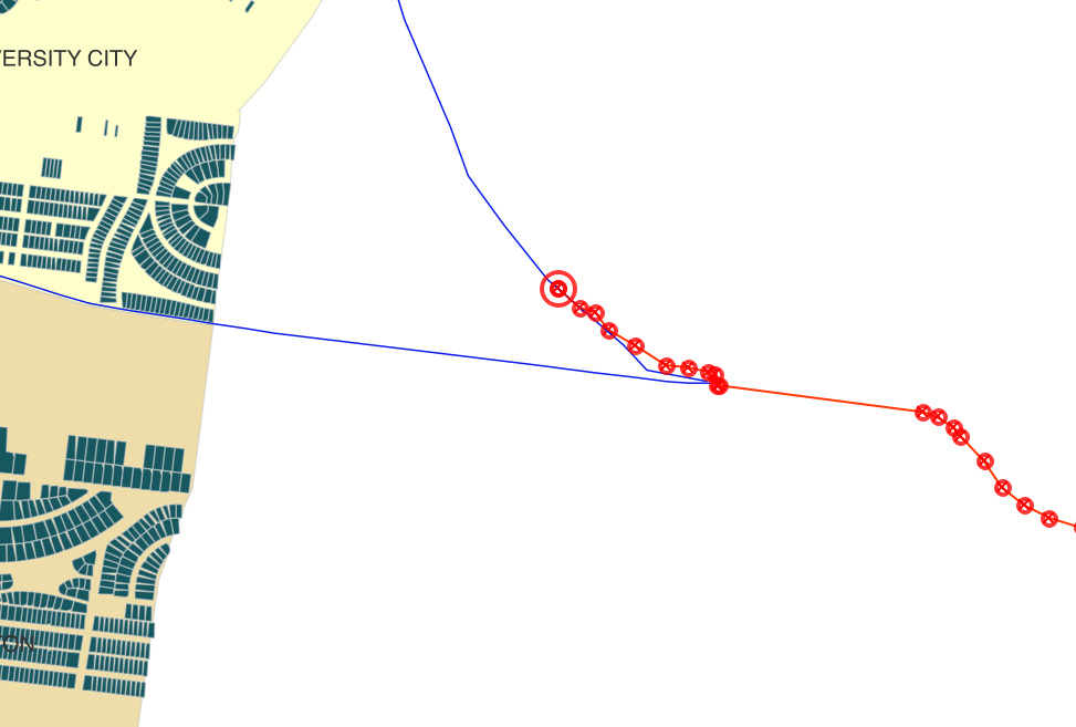
The Metrolink divides into Northwest and Southwest clearly in the map, however the geometry makes the Red Line division later than it should. We can edit the lines so we can symbolize red and blue. With the editor still on
- Select the add add feature tool
- Draw the part of the line that should be the Red line, not both lines
- Save edits
- Select the row that represents both lines and stretches into the red line
- Use the Vertex tool to select each vertex reaching into the red line and delete them
- Save edits
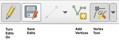
Screenshot of edit vertices tools in QGIS
In the line column, populate the fields:
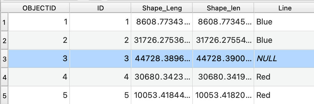
- Red
- Blue
- Blue/Red