
Chapter 4: The Nature of Geospatial Data
Adapted from Fang
How do we reduce the massive complexity of the Earth and its inhabitants so we can portray them in a GIS database and on a map? We do it by selecting the most relevant features (ignoring those we do not think are necessary for our specific research or project) and then generalizing the features we have selected. This is a geospatial data model, again there are two main types of geospatial data models, vector and raster.
Vector Data Models
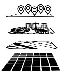
Vector data models use points and their associated [X and Y] coordinate pairs to represent the vertices of spatial features.The features are the geometries we can see and the attributes (descriptive elements) of these features are stored in a separate database management system. The geospatial information and the attribute information for these models are linked via a simple identification number that is given to each feature on a map. There are three fundamental vector geometries in GIS:
- points,
- lines, and
- polygons.
Geometries
Points
Points are zero-dimensional objects that contain only a single coordinate pair. Points are typically used to model singular, discrete features such as buildings, wells, power poles, sample locations, and so forth. Points have only the property of location. Other types of point features include the node and the vertex.
Specifically, a point is a stand-alone feature, while a node is a topological junction representing a common X, Y coordinate pair between intersecting lines (edges).
Vertices are defined as each bend along a line or polygon feature.
Lines
Points can be spatially linked to form more complex features. Lines are one-dimensional features composed of multiple, explicitly connected points. Lines are used to represent linear features such as roads, streams, faults, boundaries, and so forth. Lines have the property of length. Lines that directly connect two nodes are sometimes referred to as chains, edges, segments, or arcs.
Polygons
Polygons are two-dimensional features created by multiple lines (edges) that loop back to create a “closed” feature. In the case of polygons, the first coordinate pair (point) on the first line segment is the same as the last coordinate pair on the last line segment. Polygons are used to represent features such as city boundaries, geologic formations, lakes, soil associations, vegetation communities, and so forth. They can also be used to represent buildings and parcels. Polygons have the properties of area and perimeter. Polygons are also called areas.
Vector Data Model Structures
Vector data models can be structured many ways. We will examine two of the more common data structures here.
Spaghetti Model (sans relationships)
The simplest vector data structure is called the spaghetti data model (Dangermond 1982). In the spaghetti model, each point, line, and/or polygon feature is represented as a string of X, Y coordinate pairs (or as a single X, Y coordinate pair in the case of a vector image with a single point) with no inherent rules. One could envision each line in this model to be a single strand of spaghetti that is formed into complex shapes by the addition of more and more strands of spaghetti. It is notable that in this model, any polygons that lie adjacent to each other must be made up of their own lines or stands of spaghetti. In other words, each polygon must be uniquely defined by its own set of X,Y coordinate pairs, even if the adjacent polygons share the exact same boundary information. This creates some redundancies within the data model and therefore reduces efficiency.
Despite the location designations associated with each line, or strand of spaghetti, spatial relationships are not explicitly encoded within the spaghetti model; rather, they are implied by their location. This results in a lack of topological information, which is problematic if the user attempts to make measurements or analysis. The computational requirements, therefore, are very steep if any advanced analytical techniques are employed on vector files structured thusly. Nevertheless, the simple structure of the spaghetti data model allows for efficient reproduction of maps and graphics as this topological information is unnecessary for plotting and printing.
Topological (relationships)
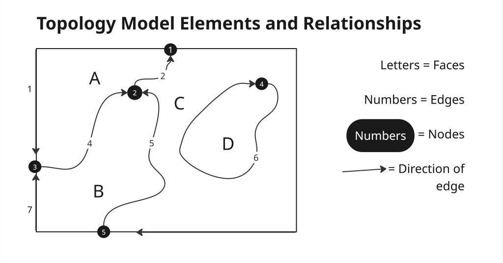
Topology in short is the definition of the relationships be between coincident geometry. In contrast to the spaghetti data model, the topological data model is characterized by the inclusion of topological information within the dataset, as the name implies. Topology is a set of rules that model the relationships between neighboring points, lines, and polygons and determines how they share geometry. Topology allows the computer to rapidly determine and analyze the spatial relationships of all its included features. In addition, topological information is important because it allows for efficient error detection within a vector dataset. For example, consider two adjacent polygons. In the spaghetti model, the shared boundary of two neighboring polygons is defined as two separate, identical lines. The inclusion of topology into the data model allows for a single line to represent this shared boundary with an explicit reference to denote which side of the line belongs with which polygon. Topology is also concerned with preserving spatial properties when the forms are bent, stretched, or placed under similar geometric transformations, which allows for more efficient projection and reprojection of map.
Three basic topological precepts that are necessary to understand the topological data model are outlined here.
First Topological Precepts
In the topological data model, nodes are the intersection points where two or more edges (lines) meet. In the case of arc-node topology, arcs have both a from-node (i.e., starting node) indicating where the edge begins and a to-node (i.e., ending node) indicating where the edge ends. In addition, between each node pair is a line segment (edge), which has its own identification number and references both its from-node and to-node.
Second Topological Precept
The second basic topological precept is area definition. Area definition states that an edge that connects to surround an area defines a polygon. Edges are used to construct polygons, and each edge is stored only once. This results in a reduction in the amount of data stored and ensures that adjacent polygon boundaries do not overlap.
Third Topological Precept
Contiguity, the third topological precept, is based on the concept that polygons that share a boundary are deemed adjacent. Specifically, polygon topology requires that all edges in a polygon have a direction (a from-node and a to-node), which allows adjacency information to be determined. Polygons that share an edge are deemed adjacent, or contiguous, and therefore the “left” and “right” side of each arc can be defined. This left and right polygon information is stored explicitly within the attribute information of the topological data model. The “universe polygon” is an essential component of polygon topology that represents the external area located outside of the study area.
Advantages of the Vector Model
Precision: Vector data models tend to be better representations of reality due to the accuracy and precision of points, lines, and polygons over the regularly spaced grid cells of the raster model. This results in vector data tending to be more aesthetically pleasing than raster data.
Scale: Vector data also provides an increased ability to alter the scale of observation and analysis. As each coordinate pair associated with a point, line, and polygon represents an infinitesimally exact location (albeit limited by the number of significant digits and/or data acquisition methodologies), zooming deep into a vector image does not change the view of a vector graphic in the way that it does a raster graphic
Storage: Vector data tend to be more compact in data structure, so file sizes are typically much smaller than their raster counterparts. Although the ability of modern computers has minimized the importance of maintaining small file sizes, vector data often require a fraction the computer storage space when compared to raster data.
Topology: The final advantage of vector data is that topology is inherent in the vector model. This topological information results in simplified spatial analysis (e.g., error detection, network analysis, proximity analysis, and spatial transformation) when using a vector model.
Disadvantages of the Vector Model
The data structure tends to be much more complex than the simple raster data model. As the location of each vertex must be stored explicitly in the model, there are no shortcuts for storing data like there are for raster models (e.g., the run-length and quad-tree encoding methodologies).
The implementation of spatial analysis can also be relatively complicated due to minor differences in accuracy and precision between the input datasets. Similarly, the algorithms for manipulating and analyzing vector data are complex and can lead to intensive processing requirements, particularly when dealing with large datasets.
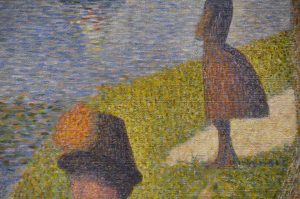
The neoimpressionist artist, Georges Seurat, developed a painting technique referred to as “pointillism” Notably, the foundation of this technology predates computers and digital cameras by nearly a century. In the 1880s, which similarly relies on the amassing of small, monochromatic “dots” of ink that combine to form a larger image.
Raster Data Model
The raster data model is widely used in applications ranging far beyond geographic information systems (GISs). Most likely, you are already very familiar with this data model if you have any experience with digital photographs. The ubiquitous JPEG, BMP, and TIFF file formats (among others) are based on the raster data model. Take a moment to view your favorite digital image. If you zoom deeply into the image, you will notice that it is composed of an array of tiny square pixels (or picture elements). Each of these uniquely colored pixels, when viewed as a whole, combines to form a coherent image.
The raster data model consists of rows and columns of equally sized cells (pixels) interconnected to form a planar surface. These pixels are used as building blocks for creating points, lines, areas, networks, and surfaces. The contrast between raster and vector models reflect the ‘pixelization’ of a raster, which would be points, lines and polygons in a vector data model. These squares are typically reformed into rectangles of various dimensions if the data model is transformed from one projection to another (e.g., from State Plane coordinates to UTM (Universal Transverse Mercator) coordinates).
Because of the reliance on a uniform series of square pixels, the raster data model is referred to as a grid-based system. Each cell in a raster grid carries a single value, which represents the characteristic of the spatial phenomenon at a location denoted by its row and column. The data type for that cell value can be either integer or floating-point.
Resolution
The area covered by each pixel determines the spatial resolution of the raster model from which it is derived. The more area covered per pixel, the less accurate the associated data values. Specifically, resolution is determined by measuring one side of the square pixel.
10m resolution: A raster model with pixels representing 10m-by-10m (or 100 square meters) in the real world would be said to have a spatial resolution of 10m;
1km resolution: a raster model with pixels measuring 1km-by-1km (1 square kilometer) in the real world would be said to have a spatial resolution of 1km; and so forth.
Care must be taken when determining the resolution of a raster because using an overly coarse pixel resolution will cause a loss of information, whereas using overly fine pixel resolution will result in significant increases in file size and computer processing requirements during display and/or analysis. An effective pixel resolution will take both the map scale and the minimum mapping unit of the other GIS data into consideration. In the case of raster graphics with coarse spatial resolution, the data values associated with specific locations are not necessarily explicit in the raster data model. For example, if the location of telephone poles were mapped on a coarse raster graphic, it would be clear that the entire cell would not be filled by the pole. Rather, the pole would be assumed to be located somewhere within that cell (typically at the center).
Raster Requirements
Imagery employing the raster data model must exhibit several properties:
- Each pixel must hold at least one value, even if that data value is zero
- If no data are present for a given pixel, a data value placeholder must be assigned to this grid cell.
- Often, an arbitrary, readily identifiable value (e.g., −9999) will be assigned to pixels for which there is no data value.
- A cell can hold any alphanumeric index that represents an attribute.
- In quantitative datasets, attribute assignation is fairly straight-forward. For example, if a raster image denotes elevation, the data values for each pixel would be some indication of elevation, usually in feet or meters.
- In qualitative datasets, data values are indices that necessarily refer to some predetermined translational rule. In the case of a land-use/land-cover raster graphic, the following rule may be applied:
- 1 = grassland
- 2 = agricultural
- 3 = disturbed
- so forth….
- Points and lines “move” to the center of the cell. As one might expect, if a 1 km resolution raster image contains a river or stream, the location of the actual waterway within the “river” pixel will be unclear.
- Therefore, there is a general assumption that all zero-dimensional (point) and one-dimensional (line) features will be located toward the center of the cell.
- As a corollary, the minimum width for any line feature must necessarily be one cell regardless of the actual width of the feature.
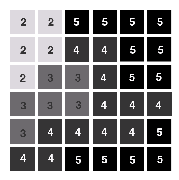
Illustration of cell-by-cell raster encoding - If it is not, the feature will not be represented in the image and will therefore be assumed to be absent.
Three (of many) models for encoding raster data from scratch:
Cell-by-cell raster encoding. This minimally intensive method encodes a raster by creating records for each cell value by row and column (This method could be thought of as a large spreadsheet wherein each cell of the spreadsheet represents a pixel in the raster image. This method is also referred to as “exhaustive enumeration.”
Run-length raster encoding. This method encodes cell values in runs of similarly valued pixels and can result in a highly compressed image file The run-length encoding method is useful in situations where large groups of neighboring pixels have similar values (e.g., discrete datasets such as land use/land cover or habitat suitability) and is less useful where neighboring pixel values vary widely (e.g., continuous datasets such as elevation or sea-surface temperatures).
Quad-tree raster encoding. This method divides a raster into a hierarchy of quadrants that are subdivided based on similarly valued pixels. The division of the raster stops when a quadrant is made entirely from cells of the same value. A quadrant that cannot be subdivided is called a “leaf node.”
Advantages of the Raster Model
Ubiquitous: Technology required to create raster graphics is inexpensive and ubiquitous. Nearly everyone currently owns some sort of raster image generator, namely a digital camera, and few cellular phones are sold today that don’t include such functionality.
Satellite Data: A plethora of satellites are constantly beaming up-to-the-minute raster graphics to scientific facilities across the. These graphics are often posted online for private and/or public use, occasionally at no cost to the user.
Simplicity: Raster graphics are the relative simplicity of the underlying data structure. Each grid location represented in the raster image correlates to a single value (or series of values if attributes tables are included). This simple data structure may also help explain why it is relatively easy to perform overlay analyses on raster data.
Interpretation: The simplicity also lends itself to easy interpretation and maintenance of the graphics, relative to its vector counterpart.
Disadvantage of the Raster Model
Storage: Raster files are typically very large. Particularly in the case of raster images built from the cell-by-cell encoding methodology, the sheer number of values stored for a given dataset result in potentially enormous files. Any raster file that covers a large area and has somewhat finely resolved pixels will quickly reach hundreds of megabytes in size or more. These large files are only getting larger as the quantity and quality of raster datasets continues to keep pace with quantity and quality of computer resources and raster data collectors (e.g., digital cameras, satellites).
Scaling: The output images are less “pretty” than their vector counterparts. This is particularly noticeable when the raster images are enlarged. Depending on how far one zooms into a raster image, the details and coherence of that image will quickly be lost amid a pixelated sea of seemingly randomly colored grid.
Reprojection: Geometric transformations that arise during map reprojection efforts can cause problems for raster graphics and represent a third disadvantage to using the raster data model. Changing map projections will alter the size and shape of the original input layer and frequently result in the loss or addition of pixels (White 2006). These alterations will result in the perfect square pixels of the input layer taking on some alternate rhomboidal dimensions. However, the problem is larger than a simple reformation of the square pixel. Indeed, the reprojection of a raster image dataset from one projection to another brings change to pixel values that may, in turn, significantly alter the output information (Seong 2003).
Analysis limitations: It is not suitable for some types of spatial analyses. For example, difficulties arise when attempting to overlay and analyze multiple raster graphics produced at differing scales and pixel resolutions. Combining information from a raster image with 10 m spatial resolution with a raster image with 1 km spatial resolution will most likely produce nonsensical output information as the scales of analysis are far too disparate to result in meaningful and/or interpretable conclusions. In addition, some network and spatial analyses (i.e., determining directionality or geocoding) can be problematic to perform on raster data.
Tabular Data
A database is a structured collection of data files. A database management system (DBMS) is a software package that allows for the creation, storage, maintenance, manipulation, and retrieval of large datasets that are distributed over one or more files. Database management normally refers to the management of tabular data in row and column format. Geospatial database management systems, alternatively, include the functionality of a DBMS but also contain specific geographic information about each data point such as identity, location, shape, and orientation.
Integrating this geographic information with the tabular attribute data of a classical DBMS provide users with powerful tools to visualize and answer the spatially explicit questions that arise in an increasingly technological society. Several types of database models exist, such as the flat, hierarchical, network, and relational models.
Hierarchical:
A hierarchical database is also a fairly simple model that organizes data into a “one-to-many” association across levels. Common examples of this model include phylogenetic trees for classification of plants and animals and familial genealogical trees showing parent-child relationships.
Network:
Network databases are similar to hierarchical databases, however, because they also support “many-to-many” relationships. This expanded capability allows greater search flexibility within the dataset and reduces potential redundancy of information. Alternatively, both the hierarchical and network models can become incredibly complex depending on the size of the databases and the number of interactions between the data points.
Relational Database Management Systems:
GIS software typically employs a relational database (Codd 1970). A relational database management system (RDBMS)
is a collection of tables that are connected in such a way that that data can be accessed without reorganization of the tables. The tables are created such that each
- column represents a particular variable which describes an object (attribute) (e.g., soil type, PIN number, last name, area)
- row contains a unique observation/instance of data for that column attribute (e.g., Delhi Sands Soils, 5555, Smith, 412.3 acres)
- each observation has a unique identifier
In the relational model, each table (not surprisingly called a relation) is linked to each other table via predetermined keys (Date 1995).
- The primary key represents the attribute (column) whose value uniquely identifies a particular record (row) in the relation (table).
- The primary key may not contain missing values as multiple missing values would represent nonunique entities that violate the basic rule of the primary key.
- The primary key corresponds to an identical attribute in a secondary table (and possibly third, fourth, fifth, etc.) called a foreign key. This results in all the information in the first table being directly related to the information in the second table via the primary and foreign keys, hence the term “relational” DBMS.
With these links in place, tables within the database can be kept very simple, resulting in minimal computation time and file complexity. This process can be repeated over many tables as long as each contains a foreign key that corresponds to another table’s primary key.
The relational model has two primary advantages over the other database models described earlier.
- Each table can now be separately prepared, maintained, and edited. This is particularly useful when one considers the potentially huge size of many of today’s modern databases.
- Tables may be maintained separately until the need for a particular query or analysis calls for the tables to be related. This creates a large degree of efficiency for processing of information within a given database.
It may become apparent to the reader that there is great potential for redundancy in this model as each table must contain an attribute that corresponds to an attribute in every other related table. Therefore, redundancy must actively be monitored and managed in a RDBMS. To accomplish this, a set of rules called normal forms have been developed (Codd 1970). [5] There are three basic normal forms.
- First Normal Form Violation refers to five conditions that must be met
-
- There is no sequence to the ordering of the rows.
- There is no sequence to the ordering of the columns.
- Each row is unique.
- Every cell contains one and only one value.
- All values in a column pertain to the same subject.
- The second normal form states that any column that is not a primary key must be dependent on the primary key. This reduces redundancy by eliminating the potential for multiple primary keys throughout multiple tables. This step often involves the creation of new tables to maintain normalization.
- The third normal form states that all nonprimary keys must depend on the primary key, while the primary key remains independent of all nonprimary keys. This form was wittily summed up by Kent (1983) [7] who quipped that all nonprimary keys “must provide a fact about the key, the whole key, and nothing but the key.” Echoing this quote is the rejoinder: “so help me Codd” (personal communication with Foresman 1989).
Joins and Relates
An additional advantage of an RDBMS is that it allows attribute data in separate tables to be linked in a post hoc fashion. The two operations commonly used to accomplish this are the join and relate.
Attribute Join
The join operation appends the fields of one table into a second table using an attribute or field that is common to both tables. This is commonly utilized to combine attribute information from one or more nonspatial data tables (i.e., information taken from reports or documents) with a spatially explicit GIS feature layer.
Requirements for a successful join
- Join fields must contain matching values
- Join fields must be the same data format (e.g., string, integer, etc.)
- Field headers must not contain spaces or special characters
- Field values are clean and standardized
- Field headers should not use reserved words (e.g., date,” “day,” “month,” “table,” “text,” “user,” “when,” “where,” “year,” or “zone”)
- Table is in an incompatible format
Spatial Join
A second type of join combines feature information based on spatial location and association rather than on common attributes.
- match each feature to the closest feature
- match each feature to the feature that it is part of
- match each feature to the feature that it intersects.
Relate
This operation temporarily associates two map layers or tables while keeping them physically separate. Relates are bidirectional, so data can be accessed from the one of the tables by selecting records in the other table. The relate operation also allows for the association of three or more tables, if necessary.
When to join or relate:
- Sometimes it can be unclear as to which operation one should use. Some considerations are:
- joins are most suitable for instances involving one-to-one or many-to-one relationships;
- joins are also advantageous because the data from the two tables are readily observable in the single output table;
- relates, on the other hand, are suitable for all table relationships (one-to-one, one-to-many, many-to-one, and many-to-many);
- relates can slow down computer access time if the tables are particularly large or spread out over remote locations.
Exercises
Exercise 4: Find the Errors in the Table
Review these tables with the ideas that you may like to join them in GIS. Identify 5 reasons these tables will NOT join.
|
objectid |
geoid |
name |
shape |
|---|---|---|---|
|
1 |
29189215301 |
Census Tract 2153.01 |
polygon |
|
2 |
29189215302 |
Census Tract 2153.02 |
polygon |
|
3 |
29189215400 |
Census Tract 2154 |
polygon |
|
4 |
29189215500 |
Census Tract 2155 |
polygon |
|
5 |
29189215600 |
Census Tract 2156 |
polygon |
|
6 |
29189215700 |
Census Tract 2157 |
polygon |
|
geoid |
Name of Area |
#people |
Date |
|---|---|---|---|
|
1500000US295101011001 |
Block Group 1, Census Tract 1011 |
115 |
2020 |
|
1500000US295101011002 |
Block Group 2, Census Tract 1011 |
0 |
2020 |
|
1500000US295101012001 |
Block Group 1, Census Tract 1012 |
29 |
2020 |
|
1500000US295101012002 |
Block Group 2, Census Tract 1012 |
107 |
2020 |
|
1500000US295101012003 |
Block Group 3, Census Tract 1012 |
23 |
2020 |
|
1500000US295101013001 |
Block Group 1, Census Tract 1013 |
16 |
2020 |
